分两个部分,第一部分,讨论时间序列数据上常用的方法,如柱状图(histograms)、曲线图(plotting),和一些能用于时间序列数据的聚合操作(group-by operations)。
第二部分,重点讨论时间序列分析相关的方法。
Familiar Methods
先从常用于时间序列数据的探索性方法。如有哪些列、取值范围。
- 某一列是否和另一列强相关?
- 某一特征均值、variance 多少?
回答这些问题,可以做一些常用的技术分析,画图、计算统计值、画柱状图、using targeted scatter plots。
同时你也需要回答面向时间的问题:
- What is the range of values you see, and do they vary by time period or some other logical unit of analysis?
- Does the data look consistent and uniformly measured, or does it suggest changes in either measurement or behavior over time?。
我们使用一些时间序列数据,做一些数据分析,并探索时间序列特有的方法和一些非时间序列方法。
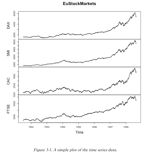
Plotting
Histograms
take a histogram of the data, also taking a histogram of the differenced data.
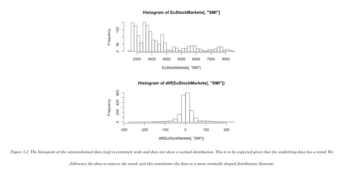
A hist() of the difference of the data is often more interesting than a hist() of the untransformed data.
After all, in a time series context, often (and particularly in finance) what is most interesting is how a value changes from one measurement to the next rather than the value’s actual measurement.
The histogram of the difference tells us that the value of the time series has gone both up (positive difference values) and down (negative difference values) about the same amount over time.
we can see from this histogram that just a slight bias in favor of positive over negative differences is what accounts for that trend.
Scatter Plots
We can use scatter plots to determine both how two stocks are linked at a specific time and how their price shifts are related over time.
In this example, we plot both cases (see Figure 3-3):
- The values of two different stocks over time
- The values of the daily changes in these two stocks over time (via differencing) with R’s diff() function
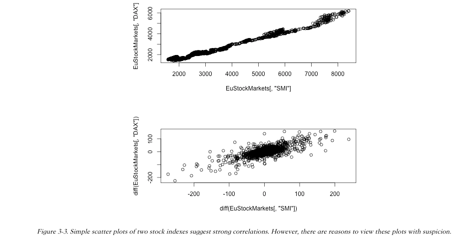
As we’ve already seen, the actual values are less informative than the differences between adjacent time points, so we have plotted the diffs in a second scatter plot. These look like very strong correlations, but the relationships are not as strong as they appear.
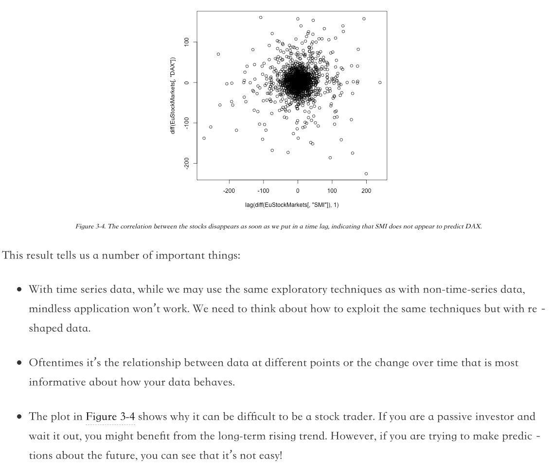
What we need to do is find out whether the change in one stock earlier in time can predict the change in another stock later in time. To do this, we shift one of the differences of the stocks back by 1 before looking at the scatter plot.
Time Series–Specific Exploratory Methods
focus on relations of values at different times in the same series.
We walk through a few concepts and related techniques used to classify time series.
We will cover the concepts and their resulting methods in order from stationarity to self-correlations to spurious correlations.
The concepts we will explore are:
Stationarity: What it means for a time series to be stationary and a statistical test for stationarity
Self-correlation: What it means to say that a time series correlates with itself and what such a correlation indicates about the underlying dynamics of the time series
Spurious correlations: What it means for a correlation to be spurious and when you should expect to run into spurious correlations
The methods we will learn to apply are:
Rolling and expanding window functions
Self-correlation functions
- The autocorrelation function
- The partial autocorrelation function
The first question you will likely ask about a time series is whether it appears to reflect a system that is “stable” or one that is constantly changing.
The level of stability, or stationarity, is important to assess because we need to know how much we should expect the system’s long-term past behavior to reflect its long-term future behavior.
Once we have assessed the “stability” (this word is not used in a technical sense here) of a time series, we try to determine whether there are internal dynamics in that series (seasonal changes, for example).
That is, we are looking for self-correlations, answering the fundamental question of how tightly past data, distant or recent, predicts future data.
Finally, when we think we have found certain behavioral dynamics within the system, we need to make sure we are not identifying relationships based on dynamics that do not in any way imply the causal relationships we wish to discover; hence, we must look for spurious correlations.
Understanding Stationarity
Many traditional statistical time series models rely on a time series being stationary.
Generally speaking, a stationary time series is one that has fairly stable statistical properties over time, particularly with respect to mean and variance.
We will walk through the concept both intuitively and with a somewhat formal definition before discussing a common test for stationarity.
INTUITION
A stationary time series is one in which a time series measurement reflects a system in a steady state. (it can be easier to rule things out as not being stationary rather than saying something is stationary. )
![]()
There are several traits that show this process(airline passengers data) is not stationary.
- First, the mean value is increasing over time, rather than remaining steady.
- Second, the distance between peak and trough on a yearly basis is growing, so the variance of the process is increasing over time.
- Third, the process displays strong seasonal behavior, the antithesis of stationarity.
STATIONARY DEFINITION AND THE AUGMENTED DICKEY–FULLER TEST

Statistical tests for stationarity often come down to the question of whether there is a unit root—that is, whether 1 is a solution of the process’s characteristic equation.1 A linear time series is nonstationary if there is a unit root, although lack of a unit root does not prove stationarity.
!(a simple intuition for what a unit root is)[/images/a-simple-intuition-for-what-a-unit-root-is.png]
Tests for determining whether a process is stationary are called $hypothesis tests$.
The $Augmented Dickey–Fuller (ADF)$ test is the most commonly used metric to assess a time series for stationarity problems.
This test posits a null hypothesis that a unit root is present in a time series. Depending on the results of the test, this null hypothesis can be rejected for a specified significance level, meaning the presence of a unit root test can be rejected at a given significance level.
待续。。。
Applying Window Functions
Understanding and Identifying Self-Correlation
Spurious Correlations
Some Useful Visualizations
1D Visualizations
2D Visualizations
3D Visualizations
More Resources
参考文献
- Practical Time Series Analysis By Aileen Nielsen